Quantification of Nitrogen-Vacancy Diamond Properties
Introduction
There has been much progress in quantum technologies within the last few decades. These quantum
technologies exploit quantum properties of material like entanglements and quantum coherence. By using
these properties it is possible to compute, communicate, and sense. A cutting-edge quantum platform within
the nitrogen-vacancy center within diamonds has huge real-world impact and implications for progress such
as being a promising sensor for magnetic fields, temperatures, and pressure. While understanding and
modeling the NV center has many purely scientific uses, its properties can be applied in medical and other
engineering settings to propel those respective fields forward.
Dr. rer. At. Dominik Bucher and Robert Allert and other researchers within the Chair of Physical
Chemistry at TUM created QuantumDiamonds. QuantumDiamonds wanted to streamline as well as
understand the process by which to build these NV diamonds so that they can produce specific types of diamonds
with desired quantum characteristics accurately and efficiently.
The main goal of this project is to understand and model different high-fidelity datasets. These datasets are both generated from diamond production and also from the measurements done on these diamonds after production. The aim ultimately is to identify and quantify the many factors that affect the NV center generation. We developed many statistical and machine learning models to optimize the diamond generation to understand latent data structures.
Rabi Data and fit methods
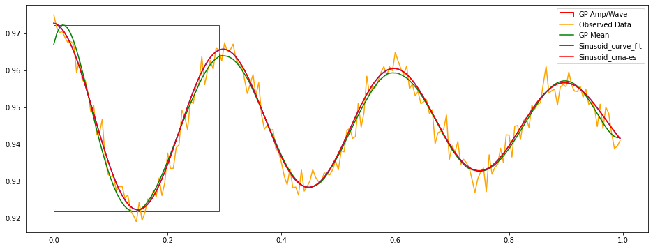
The nitrogen-vacancy (NV) center is a point defect in the diamond lattice. The first measurement of NV-diamonds is Rabi. It comes from light interacting with a particle that has both a ground state and a molecular state. This two-level system periodically exchanges energy with the light which creates the Rabi oscillation. An important thing to note is that instead of discrete absorption and emission of photons there are continuous changes in the quantum-mechanical amplitude. This amplitude indicates the probability of finding the atom in a certain state. Rabi measurements typically behave as a cosine function with exponential decay with some noise as depicted. Our main objective is then to infer their amplitudes and wavelengths as robustly as possible. To generalize and to simplify the problem, Rabi measurements are modeled as follows:
\[F(t, c, a, \tau, t_2) = c + a . cos(\pi t / \tau) . exp(-t/t_2)\]The model function takes time \(t\) and other parameters such as offset \(c\), amplitude \(a\), half of the wavelength \(\tau\),
and decaying factor \(t_2\) . Although the main focuses are on inferring the amplitude and the wavelength of a Rabi
measurement, having an offset and an exponential decay factor helps with modeling the Rabi measurements.
To model and fit data to this function, we researched and experimented with various techniques such as SG+Curve_fit, CMA-ES, Gaussian Process (GP), and finally a Neural Network with a custom loss function (NN). Here are the fit results:

Electron Spin Resonance (ESR) Data and fit methods
The other quantity we focused on was Electron Spin Resonance (ESR). ESR is a spectroscopy method for studying materials that have unpaired electrons. The unpaired electron spin is placed in a strong constant magnetic field are perturbed by a weak oscillating magnetic field and it responds by producing an electromagnetic signal with a frequency characteristic of the magnetic field on the unpaired electron. For the purpose of this analysis we assumed that ESR data was a varied length and the peaks could be modeled by (negative) Lorentzian Function. It takes time \(x\) as input and an offset \(c\), an amplitude \(a\), a peak location \(x_0\) and a width \(\Gamma\) as its parameters. The objective is then to fit those parameters given the input \(x\) and the data \(y\).
\[L(x, c, a, x_0, \Gamma) = - a. 1/\pi . 0.5 \Gamma / (x - x_0)^2 + (0.5 \Gamma)^2 + c\]Method to fit ESR
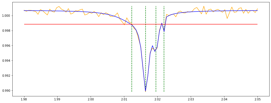
The method for computing ESR is predominantly analytical. There were attempts to use similar techniques (CMAES, GP, and NN) however we have not found any working heuristics and designs for them. Witn an analytical approach using find_peaks method in scipy.signal module combined with the curve_fit (also used in Rabi data) we were able to achieve an efficient fitting for the parameters of interest which are \(x_0\) (peak location), \(a\) (amplitude), \(\Gamma\) (width). The algorithm we have developed is called ESR_PeakFit. It takes \(x, y,\)height_factor or height, distance, max_peaks and num_iter as arguments.
ESR_PeakFit Algorithm:
- Find initial peaks \((x_0 ,y_0)\) below a certain height (either computed relative to the data or given)
- Collect the highest neighbors $$(x_1 ,y_1) of those peaks within the given distance range
- Compute initial \(a\) and \(\Gamma\) by solving Lorentzian Function given \((x_0, y_0), (x_1, y_1)\) and offset \(c\) as median of \(y\)
- Use curve_fit to fit the data \(y\) with the computed initial parameters \(c, a,\) and \(\Gamma\)

The height used to find initial peaks is either given or computed relative to the noise of the data multiplied by the height_factor. The noise is computed as \(median(|y - median(y)|)\) instead of the standard deviation asstandard deviations are biased against outliers (peaks). Our model will find more peaks if it is lower and less peaks if it is higher. The distance argument is responsible for computing neighbors of the initial peaks. One can set the maximum number of peaks to control the number of peaks and increase num_iter to run the algorithm iteratively for a smoothing purpose. In the above figure we can see an example fit of real ESR data.