Extended SIR model using Unity3D
The SIR Model
An SIR model is an epidemiological model that computes the theoretical number of people infected with a contagious illness in a closed population over time.
Number of susceptible people: \(S(t)\)
Number of people infected: \(I(t)\)
Number of people who have recovered: \(R(t)\)
The SIR system described above can be expressed by the following set of ordinary differential equations:
It is important to note that the dynamics of the infectious class depends on the following ratio: \(R_{0} = \beta / \gamma\)
Compartmental model in Unity3D
The Unity3D environment provides support for creating a lot of complex gaming scenarios. We used this capability to simulate a city. The city we built is representative of the downtown of a typical modern city.
NOTE: We chose to do the simulation in 3D with the idea to actually extend our environment and include multi-level indoor spaces. We also need to keep in mind that the spread of any disease, especially SARS-COV-2 is a 3D phenomenon so people could still be at the exact same location in x and y, but not infect each other.
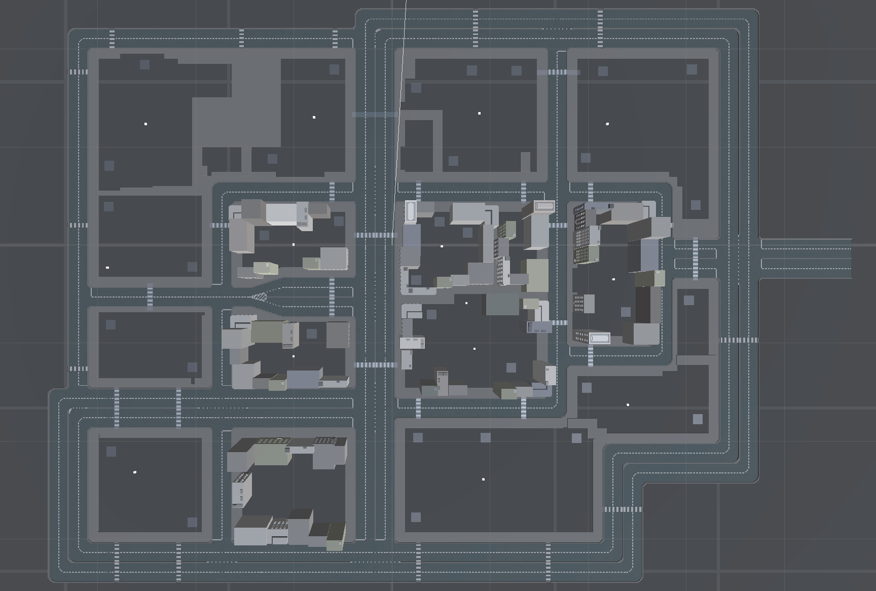
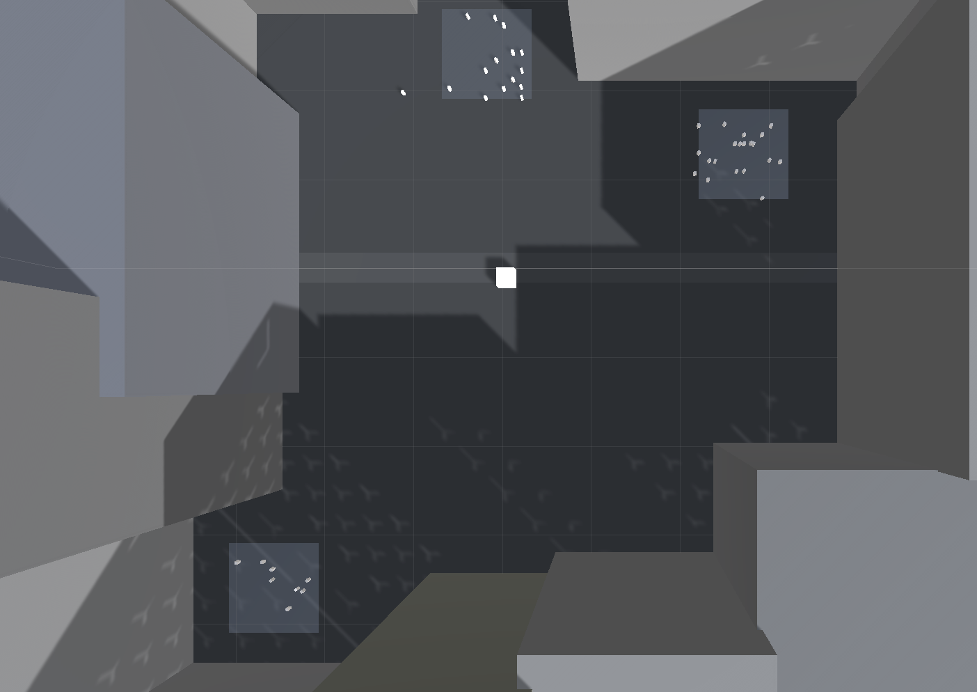
The city has 35 rectangular spawn areas from which pedestrians are spawned. It has 14 targets which the
pedestrians move to.
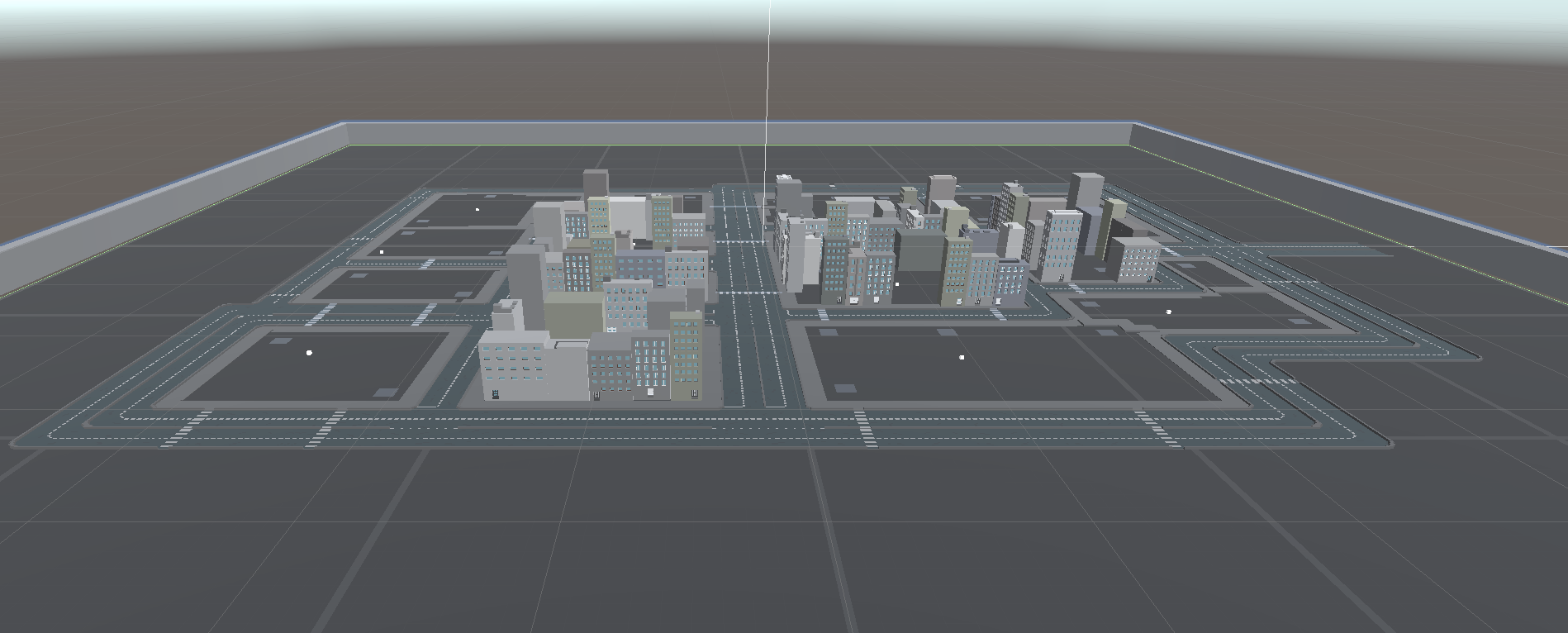
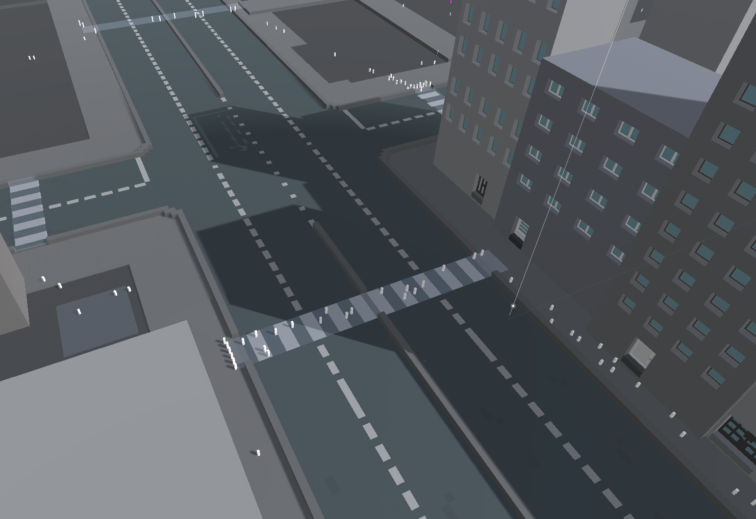
The pedestrians only move through the side walks of the streets. When they need to cross the street, they
use zebra crossings. These are typically places where there is a higher risk of infection for the pedestrians.
There are 7 states that the pedestrian can be in. They are:
- Susceptible
- Infected
- Exposed
- Infected
- Quarantined
- Recovered
- Expired
- Vaccinated The states are represented in our model using different materials.
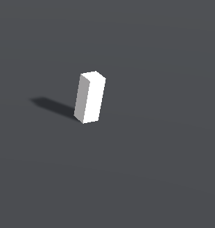

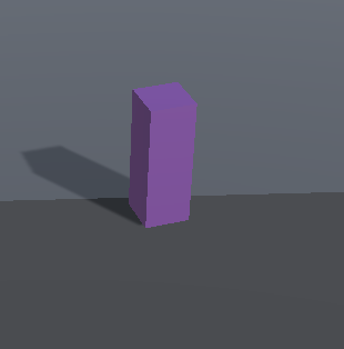
The pedestrians spawned at the spawning regions are assigned random targets. They move to these targets
one by one. During the way, they come in contact with other infected pedestrians and they get infected by
some probability. When the pedestrians are infected with the disease, they can either go back to their spawning
position to quarantine or go on with their normal life.
When the pedestrians are quarantining in their spawning positions, they cannot infect other pedestrians.
After some time, the infected pedestrians either die or recover. The probability of fatality was derived from
the studies conducted on Covid-19 If they die, they are removed from the simulation. If they recover, the
pedestrians move out of the spawning area and continue moving to different targets as they had been moving
before getting infected.
Unity NavMesh and NavMeshAgent
When we want to intelligently move pedestrians in our environment, we need to solve essentially two prob-
lems: how to reason about the level to find the destination, and then how to move there. These two problems
are tightly coupled, but quite different in nature. The problem of reasoning about the level is more global and
static, in that it takes into account the whole scene. Moving to the destination is more local and dynamic, it
only considers the direction to move and how to prevent collisions with other moving pedestrians.
In Unity the agents are described as cylinders. The walkable area is built automatically from the geometry
in the scene by testing the locations where the agent can stand. Then the locations are connected to a surface
laying on top of the scene geometry. This surface is called the navigation mesh (NavMesh for short). The
NavMesh stores this surface as convex polygons. Convex polygons are a useful representation, since we know that there are no obstructions between any two points inside a polygon. In addition to the polygon boundaries,
we store information about which polygons are neighbours to each other. This allows us to reason about the
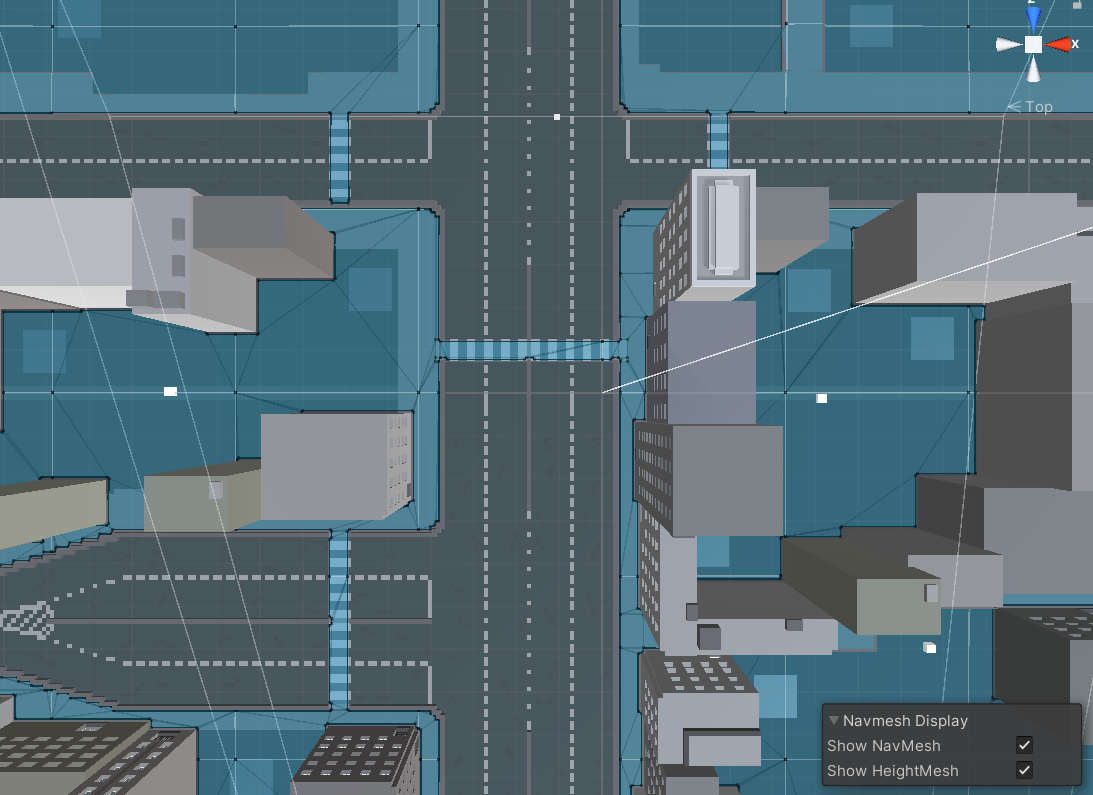
whole walkable area.Once we define all the walkable and non-walkable areas, we bake the NavMesh as shown
in the figure.
To find path between two locations in the scene, we first need to map the start and destination locations to
their nearest polygons. Then we start searching from the start location, visiting all the neighbours until we
reach the destination polygon. Tracing the visited polygons allows us to find the sequence of polygons which
will lead from the start to the destination. A common algorithm to find the path is A*
The sequence of polygons which describe the path from the start to the destination polygon is called a
corridor. The agent will reach the destination by always steering towards the next visible corner of the corridor.
When dealing with multiple agents moving at the same time, they will need to deviate from the original path
when avoiding each other. Trying to correct such deviations using a path consisting of line segments soon
becomes very difficult and error prone. The steering logic takes the position of the next corner and based on
that figures out a desired direction and speed (or velocity) needed to reach the destination. Using the desired
velocity to move the agent can lead to collision with other agents. Obstacle avoidance chooses a new velocity
which balances between moving in the desired direction and preventing future collisions with other agents
and edges of the navigation mesh. Unity is using reciprocal velocity obstacles (RVO) to predict and prevent
collisions.
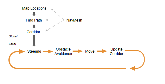
One of the most important things to understand about navigation is the difference between global and local
navigation. Global navigation is used to find the corridor across the world. Finding a path across the world is
a costly operation requiring quite a lot of processing power and memory. The linear list of polygons describing
the path is a flexible data structure for steering, and it can be locally adjusted as the agent’s position moves.
Local navigation tries to figure out how to efficiently move towards the next corner without colliding with
other agents or moving objects.
Extending the SIR Model to include Vital Dynamics
As seen earlier, Mathematical epidemic models based on the SIR model are widely used to study the spread of a disease in a population. Recently, several mathematical models have been developed to study the transmission dynamics of COVID-19. However, these models suffer from various sources of uncertainties, due to the incomplete description of the biological processes governing the disease spread, and also due to some involved parameters being poorly known. One way to mitigate these uncertainties is to constrain epidemic forecasting models with available data. These data can be combined with the model output to improve its prediction and reduce uncertainties. This process, known as data assimilation, sequentially adjusts the model state and parameters once data become available to keep the model as close as possible to the real world observations.
Model and Assimilation Scheme
We extended the SIR model to seven compartments to simulate the epidemic of COVID19. Seven state variables are considered within a population, that is, \(S(t), E(t), I(t), Q(t), R(t), D(t),\) and \(V(t)\) , denoting the number of susceptible, exposed (infected, but not yet infectious), infectious (not yet quarantined), quarantined (confirmed and infected), recovered, dead, and vaccinated cases, respectively. The disease transmission flow of the proposed model is sketched in figure shown below:
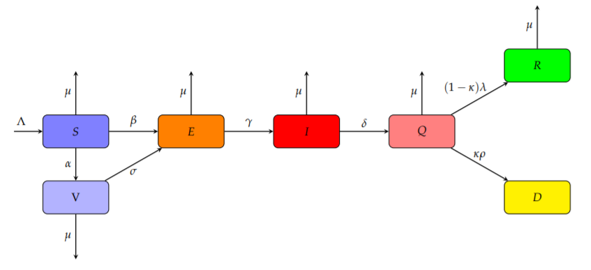
The model is then governed by the following set of nonlinear ordinary differential equations:
\[dS(t)/dt = \Lambda - \beta S(t) I(t) - \alpha S(t) - \mu S(t) ,\] \[dE/dt = \beta S(t) I(t) - \gamma E(t) + \sigma \beta V(t) I(t) - \mu E(t) ,\] \[dI/dt = \gamma E(t) - \delta I(t) - \mu I(t) ,\] \[dQ/dt = \delta I(t) - (1 - k) \lambda Q(t) - k \rho Q(t) - \mu Q(t) ,\] \[dR/dt = (1 - k) \lambda Q(t) - /mu R(t) ,\] \[dD/dt = k \rho Q(t) ,\] \[dV/dt = \alpha S(t) - \sigma \beta V(t) I(t) - \mu V(t)\]with non-negative initial conditions
\(S(0) = S0, E(0) = E0, I(0) = I0, Q(0) = Q0, R(0) = R0, D(0) = D0,\) and
\(V(0) = V0\). \(N = S + E + I + Q + R + D + V\) is the total population size.
Epidemic Equilibrium and Basic Reproduction Number of the Model
The epidemic equilibrium \(X0\) of the system is obtained by setting all the derivatives to zero with \(I = 0\), that yields to:
\[X^0 = (\Lambda/(\mu + \alpha), 0, 0, 0, 0, 0, \alpha \Lambda /(\mu(\mu + \alpha)))\]Using the next generation matrix concept, the expression for the basic reproduction number R0 turns out to be:
\[R_0 = \beta \gamma \Lambda (\mu + \alpha \sigma)/\mu (\mu + \gamma)(\mu + \delta)(\mu + \alpha)\]The basic reproduction number used to measure the transmission potential of a disease. It is the number of secondary cases or new infections produced by a single infectious individual in a completely susceptible population. An epidemic is expected to increase exponentially if \(R0\) is greater than \(1\), and to end if \(R0\) is less than \(1\).
After the creation of the compartmental model in Unity3D, we simulated different scenarios with varying conditions for quarantine, social distancing etc. and obtained the results w.r.t. the number of pedestrians who were infected, recovered, expired.

